Design space identification and exploration

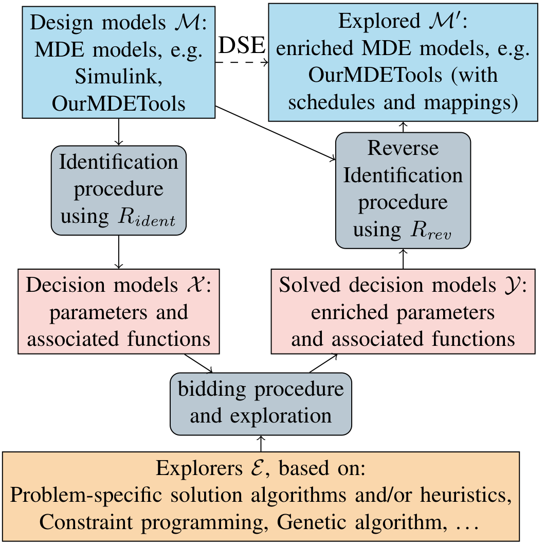
Design space identification (DSI) is a compositional and systematic approach for creating design space exploration (DSE) solutions for model-driven-engineering (MDE) models in a generic and tuneable manner. It was first proposed in this paper. Tuneablity means the capability of transparently using efficient problem-specific DSE solutions whenever possible. DSI consists of three consecutive stages (grey boxes in the Figure below) and is intuitively understood as follows:

Identification stage: This stage represents the systematic production of DSE models such as the synchronous dataflow (SDF) DSE solution of this paper from MDE inputs such as SDF3 application and platform description files. No exploration is done at this stage.
Bidding and exploration stage: This stage represents the systematic choice of the best combination of explorers (solution algorithms) and identified DSE models for the input MDE models. In other words, the choice between different design space abstractions and the solution algorithm that explores these design spaces. The chosen explorer then explores the associated chosen DSE model to enrich this DSE model with the DSE results, e.g. adding actor-to-tile mappings in the SDF DSE solution mentioned.
Reverse identification stage: This stage represents the systematic production of MDE models from the DSE solutions of the bidding and exploration stage. The systematic production includes both textual and graphical MDE models.

enhanced-position

Executing the three stages consecutively is called a flow run. The three explicit stages contrast to the first proposal, where the second and third stages are intertwined. Such enhancement is more convenient for implementation purposes because as the explicit interfaces between identification, exploration and reverse identification can be implemented in general-purpose programming languages.

From now on, we simply write DSI to refer to the enhanced version. We describe the different DSI elements (also shown in the Figure above) in the following sections; we also discuss composability and aspects of correctness.

Design models and decision models

A design model is a model used by MDE frameworks and tools, e.g. Simulink and ForSyde IO. A decision model is a collection of parameters and associated functions that potentially define design spaces, e.g. a decision model for SDFs with a topology matrix parameter and an associated function to check the existence of deadlocks.

The definitions for decision and design models are intentionally open. This openness ensures the generality and domain independence of DSI implementations such as IDeSyDe. However, every design model $M$ and decision model $X$ must provide a set of partially identified elements $\mathit{part}(X)$ and a set of partially identifiable elements $\mathit{elems}(M)$, respectively. Mathematically, $\mathit{part}(X)$ and $\mathit{elems}(M)$ can take elements from any set as long as they are the same, i.e $\mathit{part}(X) \subset \mathbb{U} \leftrightarrow \mathit{elems}(M) \subset \mathbb{U}$; in practice, $\mathbb{U}$ can be the set of strings $\mathbb{S}$ without loss of generality, since MDE components can be string encoded. For the sake of computational efficiency, unique identifiers can be used instead of encoding the entire component’s data; the component data can later be shared without jeopardising the identification procedure. IDeSyDe follows this approach.

We use $\mathit{part}(\mathcal{X})$ and $\mathit{elems}(\mathcal{M})$ as shorthand for the union of the contained $\mathit{part}(X)$ or $\mathit{elems}(M)$; that is, $\mathit{part}(\mathcal{X}) = \cup_{X \in \mathcal{X}}\mathit{part}(X)$ and $\mathit{elems}(\mathcal{M})=\cup_{M \in \mathcal{M}}\mathit{elems}(M)$.

Identification and reverse identification rules

An identification rule $r$ is a function from the input design models set $\mathcal{M}$ and any set of decision models $\mathcal{X}_i$ to a new set of decision models $\mathcal{X}_{r,i+1}$:

\[\mathcal{X}_{r,i+1} = r(\mathcal{M}, \mathcal{X}_{i})\]

as long as $r$ is monotonically increasing concerning the number of the partially identified elements of $\mathcal{M}$; that is:

\[\mathit{part}(\mathcal{X}_{r,i}) \subseteq \mathit{part}(\mathcal{X}_{r,i+1}) \subseteq \mathit{elems}(\mathcal{M})\]

Intuitively, the last equation requires that if the partially identified part of the input models does not change, the identified decision model remains the same. In other words, an identification rule at step $i+1$ cannot partially identify less elements than it did at step $i$ the recurrence equation. Checking that a function $r$ satisfies monotonicity automatically is difficult as it ultimately requires checking if $r$’s implementation never violates the condition for any input. An alternative to ensure $r$ is monotonic is to define a set of identification rule function templates that are monotonic by construction. This is yet to be researched and developed.

A reverse identification rule $\rho$ is a function from the input design models set $\mathcal{M}$ and the set of explored decision models $\mathcal{Y}$ to a new set of explored design models $\mathcal{M}_{\rho}'$:

\[\mathcal{M}_{\rho}' = \rho(\mathcal{Y}, \mathcal{M})\]

Unlike identification rules, reverse identification rules have no requirements relating its inputs and outputs. This considerably reduces the initial effort for implementing a new $\rho$ when the input and output MDE frameworks are different. An example case is taking Simulink models as input design model and producing ForSyDe IO design models as output. In these cases, a requirement such as monotonicity potentially requires $\rho$ to be a complete model-to-model transformation.

Explorers

An explorer $E$ is a collection of decision and optimisation methods that explore the design space of decision models. These methods range from generic decision and optimisation frameworks such as constraint programming to problem-specific heuristics. Consequently, an explorer can be incapable of solving a decision model if the decision model is not compatible with the explorer’s method.

This is represented with a function $\mathit{able}_E(X)$ for every $E$ which is true if $E$ can explore $X$ and false otherwise. Additionally, a function $\mathit{explore}_E(X)$ exists for every $E$ that returns a set of explored decision models $\mathcal{Y}$. The reason both $\mathit{explore}_E(X)$ and $\mathit{able}_E(X)$ exists is to distinguish when $\mathcal{Y}$ is empty because no solution exists, and when $\mathcal{Y}$ is empty because $E$ cannot explore $X$.

Different explorers may display different exploration properties for the same decision model. For example, one explorer is the most accurate but also the slowest for a decision model. Note that exploration properties are not the same as performance metrics but characteristics of the exploration method itself. We remark that exploration properties can be estimates. For example, the exploration property “average time to find a first feasible solution” for the SDF CP solution mentioned could be estimated as an expression on the size of actor and channels of the input SDF applications.

These properties are represented through biddings. The bidding of $E$ for a decision model $X$, $\mathit{bid}_E(X)$, is a set of pairs in $\mathbb{S} \times \mathbb{R}$ with non-negative real entries. Biddings define a dominance relation that can be exploited to automate the choice of the best biddings. For every two distinct $(E, X)$ and $(E', X')$ where $\mathit{able}_E(X)$ and $\mathit{able}_{E'}(X')$ are both true, we say that $(E, X)$ dominates $(E', X')$ if either:

$\mathit{part}(X') \subset \mathit{part}(X)$; or,
$\mathit{part}(X') = \mathit{part}(X)$ but $\mathit{bid}_E(X)$ and $\mathit{bid}_{E'}(X')$ have equal entries string-wise but the former is smaller number-wise.

The first condition ensures dominance when $X$ partially identifies more elements than $X'$ in accordance with the DSI approach; the second condition ensures dominance for the explorer $E$ when it is a better explorer for comparable decision models.

First stage: identification procedure

In the first stage, a set of decision models $\mathcal{X}$ is identified from the input design models set $\mathcal{M}$ given a set of identification rules $R_{\mathit{ident}}$. This identification is performed stepwise through the identification procedure recurrence relation:

\[\mathcal{X}_{i+1} = \mathcal{X}_{i} \bigcup_{r \in R_{\mathit{ident}}} r(\mathcal{M}, \mathcal{X}_i)\]

The identification procedure is performed until a fix-point $\mathcal{X}$ is reached; that is, $\mathcal{X} = \mathcal{X}_{i+1}$ when $\mathit{part}(\mathcal{X}_{i+1}) = \mathit{part}(\mathcal{X}_{i})$, as outlined by the recurrence equation presented previously. This fix-point exists due to the monotonicity requirement, and the resulting identified decision model set $\mathcal{X}$ is used in the next stage.

Note that the initial set $\mathcal{X}_0$ is not specified. This is because the recurrence equation is incremental; the first execution for a $\mathcal{M}$ starts with $\mathcal{X}_0 = \emptyset$, but the equation can be repeated with the resulting $\mathcal{X}$, or any intermediate $\mathcal{X}_i$, to achieve the same $\mathcal{X}$ fix-point for $\mathcal{M}$.

An identification rule returns a set of identified decision models instead of a single decision model as defined in the first proposal. However, these two definitions are conceptually equivalent since identification rules in the first proposal also progressively “partially identify more elements of $\mathcal{M}$ by taking previously partially identified $X \in \mathcal{X}$”.

Second stage: bidding procedure and exploration

In the second stage, a set of explorers $\mathcal{E}$ bid for the identified decision models and the winning bid proceeds to exploration. The bidding procedure may result in multiple biddings do not dominate each other; if there is more than one bidding, they cannot be compared by construction, and one is randomly chosen.

Mathematically, the set $\mathcal{B} \subset \mathcal{E} \times \mathcal{X}$ of dominating bids is computed via the dominance relation by keeping only the dominant bids:

\[\mathcal{B} = \left\{ \begin{gathered} (E, X) \\ \in \mathcal{E} \times \mathcal{X} \end{gathered} \middle\vert \begin{aligned} \nexists & (E', X')\in \mathcal{E} \times \mathcal{X} \setminus \{(E, X)\}, \\ &(E, X) \text{ dominates } (E', X') \end{aligned} \right\}\]

then, a bid $(E, X) \in \mathcal{B}$ is chosen and so that $\mathit{explore}_E(X)$ returns a set $\mathcal{Y}$ of explored decision models for the last stage.

Third stage: reverse identification procedure

Despite their conceptual analogy, the reverse identification procedure is simpler than the identification procedure. This is because the input explored decision models $\mathcal{Y}$ are already dominant, which entails that all the elements required to obtain the explored design model are already present in $\mathcal{Y}$. Thus, one identification step is enough and a fix-point-based procedure like the identification one is unnecessary. The final explored design model set $\mathcal{M}'$ is given by the union of the results of the given set of reverse identification rules $R_{\mathit{rev}}$:

\[\mathcal{M}' = \bigcup_{\rho \in R_{\mathit{rev}}} \rho(\mathcal{Y}, \mathcal{M})\]

We choose the word “reverse” instead of “inverse” as reverse identification rules are not inverse mathematical functions of identification rules. By bidding, we mean the process where different explorers share exploration characteristics and compete to explore a decision model.

Composability and correctness aspects

The DSI composability is centred around identification rules, explorers and reverse identification rules. Extending a DSI-based DSE tool, such as IDeSyDe, is equivalent to adding a new identification rule, explorer, or reverse identification rule. This is possible because the definitions presented here do not require explicit dependencies between themselves or across different stages, nor do they require explicit dependencies on a subset of design or decision models. Due to this loosely-coupled nature, the backwards compatibility of tools like IDeSyDe is systematically guaranteed if extensions are strictly additive.

Since the decision and design model definitions are open, correctness is only well-defined on a model-by-model basis. However, as a composable approach, the conservation of correctness can be discussed and analysed.

Concretely, every decision model has invariants that are always valid, e.g. for SDF decision models, actors only connect through channels, not directly. In this sense, a correct identification rule always produces decision models satisfying their invariants. Design models and reverse identification rules can be discussed analogously as MDE frameworks typically have their invariants and assumptions. Because explorers are a collection of methods, they are correct if such methods are sound and complete.

Automatically verifying these notions of correctness is difficult; for the same reasons verifying monotonicity cannot be easily verified automatically. However, verification can be avoided by defining decision and design models so that their invariants are valid by construction. For example, a decision model for tiled-based multicore hardware without parameters or associated functions for shared-memory elements avoids checking if the model contains shared-memory elements. Currently, IDeSyDe follows this correct-by-construction approach as much as possible and provides documentation when invariants must be enforced via (reverse) identification rules.