ForSyDe-SystemC

The SystemC implementation of ForSyDe

The ForSyDe-SystemC Tutorial for the Continuous-Time MoC

This tutorial is a walk-through for modeling systems in the Continuous-Time (CT) Model of Computation (MoC) using the ForSyDe-SystemC library. It assumes that the user has already installed the SystemC and the ForSyDe-SystemC libraries and knows how to build and run a model on her computer. The basic concepts for modeling systems using ForSyDe-SystemC are already covered in the SY MoC tutorial. Hence, the reader is encouraged to read it before this tutorial.

In ForSyDe-SystemC, a system is modeled as a hierarchical process network where processes communicate only via signals, making it similar to the data-flow style of modeling. We will introduce different elements of the CT MoC in ForSyDe-SystemC with an example.

In order to avoid confusion, note that although ForSyDe-SystemC uses the SystemC kernel to simulate the models, the modeling style is different from SystemC. Many elements of the SystemC language are not present¹ in ForSyDe-SystemC, and the ones which are used may appear in a different terminological context.

Modeling

A synopsis of the low pass filter system is illustrated in the picture below. It contains 7 modules, in a single level of hierarchy, which are to be modeled consequently.

CT Signals

In the CT MoC, signals are defined using the class ForSyDe::SY::CT2CT (or ForSyDe::CT::signal). A CT signal is a function from the time domain to the value domain and the tokens carried by a CT signal are sub-signals which are functions from a sub-range of the time domain to the value domain. There is a helper (template) class ´ForSyDe::sub_signal´ which is used to represent the tokens in a sub-signal.

The signals used to interconnect the processes in the above example can be defined as:

ForSyDe::CT::signal cosSrc, NoiseSrc1, NoiseSrc2, filtInp, filtOut;

These signals carry tokens of type sub_signal. Usually the normal user of the ForSyDe-SystemC library does not see the sub_signal class and writes her functions directly in the value domain.

Signal Source

The signal source is a cosine wave generator with a frequency of 5 HZ. The cosine signal is defined with a frequency of 5 HZ over time period [0.0s, 1.0s]. A signal source named cosine1 is instantiated from the CT::cosine class using the helper function CT::make_cosine.

CT::make_cosine("cosine1", endT, CosPeriod, 1.0, cosSrc);

cosSrc the signal to which the output is connected.

Gaussian Noise

The noise is defined as a Gaussian noise with a variance of 0.01 and the mean value 0. A sampling period of 1 ms is chosen to identify how long each generated random value should stretch in time. This source is created using the CT::gaussian class in the library and is instantiated and initialized using the helper function make_gaussian.

CT::make_gaussian("gaussian1", 0.01, 0, sc_time(1, SC_MS), NoiseSrc1);

NoiseSrc1 the signal to which the output is connected.

Addition Module

Caused by the additive noise, the actual signal is the cosine signal plus the interference effects from the environment. A module with two-input and one-output is instantiated from the library provided CT::add class, for signal addition operations.

auto add1 = CT::make_add("add1", filtInp, cosSrc, NoiseSrc1);
add1->oport1(NoiseSrc2);

NoiseSrc1 (one of) the signal(s) to which the output is connected while cosSrc and NoiseSrc1 are the input signals. Unlike the previous cases, we need to connect the output port of add1 to two signals. This is accomplished by first assigning the returned process add1 to a temporary variable, and then binding the output port in the SystemC style to the second signal. The auto keyword is a newly-added feature of the latest C++11 standard which in this case automatically infers the type of the add1 process (pointer).

In general, one can also use the CT::comb2 module and customize it by implementing its pure virtual function member in order to implement any desired function over the two input signals.

Low Pass Filter

A low-pass filter with the transfer function

is designed to pass low-frequency signals but attenuates the Gaussian noise with frequencies higher than the cutoff frequency ‘‘freq_cutoff’’. The numerator and denominator coefficients are specified as vectors nums and dens. A maximum step size samplingPeriod for the adaptive Runge-Kutta solver in digital domain is chosen. The filter process is instantiated as:

CT::make_filter("filter1", nums, dens, samplingPeriod, filtOut, filtInp);

Signals Tracing

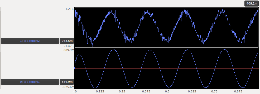
Tracing of CT signals is supported by processes instantiated from the CT::traceSig class. The result will be a file placed beside the simulator executable with the same name as the module and can be plotted using a program like ‘‘gaw’’.

Let us put all the pieces together and define the top level of the system.

#include <forsyde.hpp>

#include "globals.hpp"

using namespace sc_core;
using namespace ForSyDe;

SC_MODULE(Top)
{
    CT::signal cosSrc, NoiseSrc1, NoiseSrc2, filtInp, filtOut;
    
    SC_CTOR(Top)
    {
        
        CT::make_cosine("cosine1", endT, CosPeriod, 1.0, cosSrc);
        
        CT::make_gaussian("gaussian1", 0.01, 0, sc_time(1, SC_MS), NoiseSrc1);
        
        auto add1 = CT::make_add("add1", filtInp, cosSrc, NoiseSrc1);
        add1->oport1(NoiseSrc2);
        
        CT::make_filter("filter1", nums, dens, samplingPeriod, filtOut, filtInp);
        
        CT::make_traceSig("report1", sc_time(100,SC_US), filtOut);
        
        CT::make_traceSig("report2", sc_time(100,SC_US), NoiseSrc2);
    }
   
};

The globals.hpp file is defined as:

#ifndef GLOBALS_HPP
#define GLOBALS_HPP

#include <forsyde.hpp>
using namespace sc_core;
using namespace ForSyDe;

// Period of the cosine wave
sc_time CosPeriod = sc_time(200,SC_MS);
// The end time of the cosine wave signal
sc_time endT = sc_time(1.0,SC_SEC);

double cutoffFreq = 2.0/(CosPeriod.to_seconds());
// Sampling period of the solver for filter
sc_time samplingPeriod # sc_time(100,SC_US);

std::vector<CTTYPE> nums = {1.0};
std::vector<CTTYPE> dens = {1.0/(M_PI*cutoffFreq), 1.0};

#endif

Compilation and Simulation

To run the simulation, we need to instantiate the top level composite process and run the SystemC simulation kernel.

#include "top.hpp"

int sc_main(int argc, char **argv)
{
    top top1("top1");

    sc_start();
        
    return 0;
}

Compilation of the project is just like any other C++ application. Depending on the way you have built your SystemC library (statically or dynamically), you compile the code and link against SystemC to yield a single executable file. By running the resulting executable file, we are in fact simulating our system. Below you can see a snapshot from the gaw tool which is used to plot the output traces of the simulation.

or in better words, are not allowed to be used ↩